Uniaxial ferromagnet

The model description

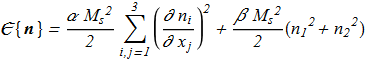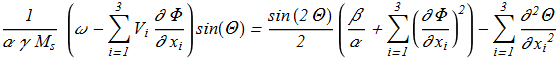The only difference from the Heisenberg model is an additional term in the functional - the energy of uniaxial magnetic anisotropy: (1.1) where (1.2) Governing equations: (1.3) (1.4)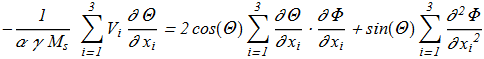 For the case of axially symmetric solitons propagating along the axis of precession: (1.5) (1.6) (for details, see Heisenberg model).

The first works

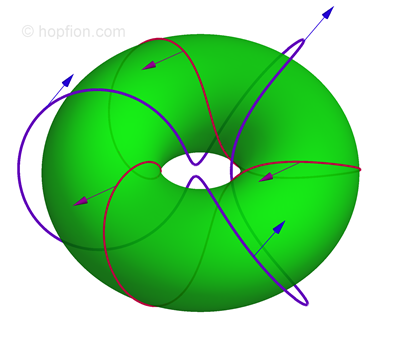
In work [I.E. Dzyloshinskii and B.A. Ivanov "Localized topological solitons in a ferromagnet", JETP Lett. 29, 540 (1979) ref] the authors showed that in a uniaxial ferromagnet, stationary precessional hopfion can exist (2.1)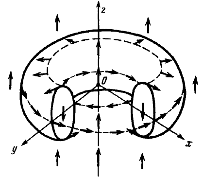 The velocity may be zero, and the frequency - is positive: (2.2) Hobart-Derrick theorem forbids the existence of three-dimensional solitons in the fully static case: (2.3) A very important difference from the isotropic Heisenberg model is the appearance of the scale parameter: (2.4) The most common properties of precessional hopfions were discussed in several subsequent studies [A. M. Kosevich, B. A. Ivanov and A. S. Kovalev, "Nonlinear Magnetization Waves. Dynamical and Topological Solitons", Nauk. Dumka, Kiev, (1983), (in Russian)], [A.M. Kosevich, B.A. Ivanov, A.S. Kovalev "Magnetic Solitons", Phys. Rep. 194, 117 (1990) ref].

The results of recent years

In the paper [N.R. Cooper " 'Smoke Rings' in Ferromagnets", Phys. Rev. Lett. 82, 1554 (1999) ref; arXiv:cond-mat/9901037v1] (for details, see Heisenberg model) was announced that the published numerical calculation is performed also for an anisotropic system, but the publication was not followed.

In the paper [P. Sutcliffe "Vortex Rings in Ferromagnets", arXiv:0707.1383v1; Phys. Rev. B 76, 184439 (2007) ref], numerical calculations were performed for the anisotropic case also, but for the anisotropic case a stable hopfion is not found. The author argues that the reason for this is the instability to axial perturbations for the anisotropic system. However, this conclusion can not be considered correct on the basis of the results. Stability can still occur, but the magnitude of the perturbation must be less than the author has used in the calculations. It is also possible that the number of nodes in the grid is too small or the distance between them is too large. The distance between two adjacent nodes in the lattice used: (3.1)

In the paper [A.B. Borisov, F.N. Rybakov "Stationary Precession Topological Solitons with Nonzero Hopf Invariant in a Uniaxial Ferromagnet", JETP Lett. 88, 264 (2008) ref, arXiv:0810.5658v1], the authors obtained the numerical solutions for stationary precessional toroidal hopfions with H=2,3,4. Dependence of the energy and energy density from precession frequency was determined. From the paper, it follows that the hopfions have thin structural features and for their calculation it is necessary to use a very dense grid, and the criterion {3.1} is too coarse. This feature is stronger for smaller Hopf indices. For H = 1, the authors even with all the symmetries are not able to get the result.

In a subsequent article [A.B. Borisov, F.N. Rybakov "Dynamical Toroidal Hopfions in a Ferromagnet with Easy-Axis Anisotropy", JETP Lett. 90, 544 (2009) ref, arXiv:0911.0451v1], studies have been generalized to the case of non-zero velocity. An interesting statement about the coexistence of two types of solitons with the same frequency, speed and Hopf index, but with different energies: (3.2)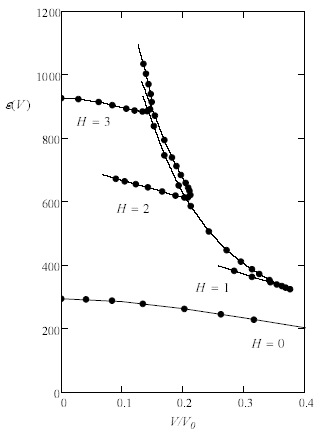

Still unsolved problems

1. Analytical soliton solution in 3D for set of equations {1.3} - {1.4}, even in case {1.5} - {1.6}, for Q>0
2. Stationary hopfion with topological charge H=1
3. Hopfions without axial symmetry
4. Other types of anisotropy

Problems that should be resolved before attempt an experimental observation

1. Accounting for the effects of magnetic dipole-dipole interaction
2. In fact, because of energy dissipation, dynamic solitons will quickly fade. But perhaps there may be modes of the "pump" or the "capture" of the solitons, which will significantly increase the lifetime. These modes represent the change in time the external magnetic field, possibly inhomogeneous in space, but it should be feasible. These modes can be found theoretically from the dynamic evolution equation with dissipation. (Apparently only by numerical methods)

This page is not complete and if you find inaccuracies, if you have any comments or additional material - do not hesitate to contact us.